Text analysis of last meals
Examining favorite foods through last meal requests
Last summer I toured an 1800s era state penitentiary which included the requisite walk-through of the execution room. The tour guide spoke about the prisoners’ pasts and spent considerable time discussing their last meals. Besides the obvious morbid thoughts of death and questions on the ethics of capital punishment, it struck me that these meals could serve as a great proxy for exploring peoples’ favorite foods.
Recently I came across the last meals Wikipedia page which includes a table of 130 U.S. condemned prisoners’ choices for their final feast. This is a great, approachable dataset to test out some text analysis tricks and unearth any patterns.
Summary findings
Ice cream. That’s what everyone wants. After scraping, cleaning, and tokenizing the text, the most common items are also the most obvious: ice cream, french fries, steak, pizza, and fried chicken. These five show up in 66% or in 85 of the cases.

Notably, these top five foods occur 131 times, indicating there are some repeats within a request and/or co-occurrences. That’s not all that informative, though. There’s a smarter way to explore trends within this dataset. We can look for similarities and differences in meals using cosine similarity. It allows us to quantify the similarity of vectors based on the count of similar instances between two vectors. I.e. how often do foods co-occur within a last meal. Higher scores will be given to words that co-occur more often signifying strength of the relationships. Performing this for each pair of items, these scores can be graphed to provide a visual sense of any patterns.

There are two clear communities. In the top-left section, simple comfort food such as mashed potatoes, gravy, tea, peas, and rice all naturally go together. In the center-right section, indulgent food such as hamburger, onion rings, fried chicken, and steak are grouped. Intuitively, cheese is stuck right in the middle of these two groups. I interpret this as it’s the great equalizer, almost everyone loves cheese and it goes with almost any food.
The analysis process
Exploring this corpus is a complex, multi stage process where significant cleaning decisions need to be made. Once finished, the data is relatively simple to anlayze.
- Cleaning the data
- Analyzing the data
If you just want the R code, go to github.com/joemarlo/Last-meals
Scraping the tables
Scraping the tables off Wikipedia is simple using the rvest package. It’s similar to the ubiquitous Beautiful Soup package for Python. We can pull the html quickly, search for the nodes that represent the tables on the website and then do some wrangling to get the data into a tidy format.
# scrape the table
tables <- read_html('https://en.wikipedia.org/wiki/Last_meal') %>%
  html_nodes(xpath = '//table[contains(@class, "sortable")]') %>%
  html_table() %>%
  .[[4]]
We need to remove cases of inmates that didn’t request a meal or received a meal that was not requested. We’re interested in what people wanted as their last meal, not necessarily what they received. This also removes some cases such as prisoner’s requesting communion in lieu of a meal.
excl.names <- c("David Mason", "Odell Barnes", "Philip Workman", "Ledell Lee")
US.table <- US.table[!(US.table$Name %in% excl.names),]

head(US.table)
# A tibble: 6 x 6
  Name        Crime     State   Year Method.of.Dispa… Requested.Meal
  <chr>       <chr>     <chr>  <dbl> <chr>            <chr>
1 Adam Kelly… Murderer  Texas   2016 Lethal injection "Beef soft tacos, Spanish rice, salsa, mixed greens…
2 Aileen Wuo… Serial k… Flori…  2002 Lethal injection "Declined a special meal, but had a hamburger and o…
3 Allen Lee … Murderer  Flori…  1999 Electrocution    "350-pound \"Tiny\" Davis had one lobster tail, fri…
4 Alton Cole… Spree Ki… Ohio    2002 Lethal injection "Well done filet mignon smothered with mushrooms, f…
5 Andrew Lac… Murderer  Alaba…  2013 Lethal injection "Turkey bologna, French fries, and grilled cheese."
6 Ángel Niev… Murderer  Flori…  2006 Lethal injection "Declined a special meal. He was served the regular…
Tokenizing
The first challenge is separating all the food related words and phrases from the non-food. This could be quite easy or quite difficult depending on meal description. For example,
“Salmon and potatoes.”
is straightforward. Each item is a food word. We just need to extract the words ‘salmon’ and ‘potatoes.’
Using the tidytext package we can pull out the words (or unigrams) using unnest_tokens() and remove the stop words (‘and’, ‘is’, ‘a’, etc.) by anti-joining with the built-in stop_words dataset.
parsed.words <- US.table %>%
  select(Name, Requested.Meal) %>%
  unnest_tokens(output = word, input = Requested.Meal) %>%
  anti_join(stop_words, by = "word")

head(parsed.words)
# A tibble: 6 x 2
  Name            word
  <chr>           <chr>
1 Adam Kelly Ward beef
2 Adam Kelly Ward soft
3 Adam Kelly Ward tacos
4 Adam Kelly Ward spanish
5 Adam Kelly Ward rice
6 Adam Kelly Ward salsa
However, there’s two major issues: 1. it’s not finding items that consist of one or more words like “ice cream” and 2. it’s finding irrelevant words like “wishing.”
Now consider the following example:
“Morrow requested a last meal of a hamburger with mayonnaise, two chicken and waffle meals, a pint of butter pecan ice cream, a bag of buttered popcorn, two all-beef franks, and a large lemonade.”
How would you systematically go through this and decide which words or series of words to keep?
First, let’s replace the unigram method with uni-, bi- and trigrams. This will return all permutations of 1, 2, and 3 word phrases. In the above example, the four word phrase ‘butter pecan ice cream’ would return the follow variations:
butter
butter pecan
butter pecan ice
pecan
pecan ice
pecan ice cream
ice
ice cream
cream
# tokenize the meals
parsed.ngrams <- US.table %>%
  select(Name, Requested.Meal) %>%
  unnest_tokens(output = word, input = Requested.Meal, token = "ngrams", n = 3, n_min = 1) %>%
  anti_join(stop_words, by = "word")
Foodbase corpus
Second, we need a way to understand if the word is in fact food- or meal-related. The easiest method is to compare against a pre-processed list. Finding a dictionary of food related words was more difficult than I anticipated. I finally found the FoodBase corpus, a collection of 22,000 recipes with 274,000 ‘food entities’ in XML format. Each recipe has a list of its ingredients that can be easily extricated, deduped, and then turned into a list of ‘food’ items. This will serve as a master list of food-related words. Any items that are in our dataset but not in this dataset will be removed. I’ve also manually excluded a few additional words that made it through such as ‘meal’, ‘food’, ‘drink’, etc., and added ‘coke’ and ‘pepsi’ as I think these are relevant.
# import the food words from the Foodbase corpus
food.words  <- read_xml('Data/Foodbase/FoodBase_uncurated.xml') %>%
  xml_find_all(xpath = "/collection/document/annotation/text") %>%
  xml_text() %>%
  unique() %>%
  enframe(value = "word") %>%
  select(-name) %>%
  str_to_lower()

# remove copmmon condiments from the food words list
excl.words <- c("meal", "food", "snack", "drink", "double", "sauce", "ketchup", "cups",
                "mustard", "mayonnaise", "mayo", "sour cream", "onion", "meat",
                "onions", "pepper", "butter", "ranch", "ranch dressing")
food.words <- food.words[!(food.words %in% excl.words)]

# add additional one-off words
food.words <- append(food.words, c("coke", "pepsi"))
parsed.ngrams <- parsed.ngrams %>%
  filter(word %in% food.words)
head(parsed.ngrams)
# A tibble: 6 x 3
  Name            word          stem
  <chr>           <chr>         <chr>
1 Adam Kelly Ward beef          beef
2 Adam Kelly Ward tacos         taco
3 Adam Kelly Ward rice          rice
4 Adam Kelly Ward salsa         salsa
5 Adam Kelly Ward corn          corn
6 Adam Kelly Ward refried beans refried bean
Deduping
After filtering for food-related words, we are left with pecan ice cream, ice, ice cream, and cream in the above example. Much improved over the just the ngrams but it’s double counting ice. It appears in both ice and ice cream. We can remove these duplicates on a meal-basis by excluding words that exist in longer strings. E.g. exclude “ice” if there is another string like “ice cream” but keep “ice cream.” We’ll have to make a judgement call to exclude three word phrases at this point. I believe it’s more important to include ice cream than pecan ice cream because another meal may include chocolate ice cream and it’s more important to get an accurate count of ice cream than it is to include modifiers.
# split the $word with more than one word into a list
#  then split the dataframe by $Name
# remove unrelated words
name.groups <- parsed.ngrams %>%
  mutate(word = str_split(word, pattern = " ")) %>%
  group_by(Name) %>%
  group_split()

# check to see if the $word is contained within
#  another $word for that $Name
deduped.ngrams <- lapply(name.groups, function(group) {

  # if only one unique word then return that one word
  if (length(unique(group$word)) == 1) {
    non.duplicates <- group$word[1]
  } else{
    # for groups that have more than one row check to
    #   see if a word is contained in another row
    duplicate.bool <-
      sapply(1:length(group$word), function(i) {
        x <- group$word[i]
        lst <- group$word
        lst <- lst[!(lst %in% x)]
        word.in.list <- sapply(lst, function(y) {
          x %in% y
        })
        return(sum(word.in.list) == 0)
      })

    non.duplicates <- group$word[duplicate.bool]

    # remove $words that are more than two
    #  individual words (e.g. "chocolate ice cream") b/c
    #  these will be captured in "ice cream"
    non.duplicates <- non.duplicates[sapply(non.duplicates, length) <= 2]
  }
  return(group %>% filter(word %in% non.duplicates))
}) %>% bind_rows()
rm(name.groups)

# unlist the word column
deduped.ngrams <- deduped.ngrams %>%
  rowwise() %>%
  mutate(word = paste0(word, collapse = " ")) %>%
  ungroup()
Manual checks
I like to do a quick manual check to see if there are any obvious issues that the previous methods didn’t correct. An easy way to do this is to find the best matches between the words based on string edit distance. We can wrap stringdist::stringsim() in a custom function and have it pick out the top five matches. If any of these matches are essentially the same as the word, then our previous methods didn’t work well.
get_top_matches <- function(current.word, words.to.match, n = 5){
  # function returns that top n matches of the current.word
  #   within the words.to.match list via fuzzy string matching

  scores <- stringsim(current.word, words.to.match, method = "osa")
  words.to.match[rev(order(scores))][1:(n + 1)]
}

# apply the function across the entire list to generate a data.frame
#  containing the current.name and it's top 5 best matches
lapply(deduped.ngrams$word,
                      get_top_matches,
                      words.to.match = unique(deduped.ngrams$word)) %>%
  unlist() %>%
  matrix(ncol = 6, byrow = TRUE) %>%
  as_tibble() %>%
  setNames(c("Current.word", paste0("Match.", 1:5))) %>%
  head()
# A tibble: 6 x 6
  Current.word Match.1    Match.2   Match.3    Match.4 Match.5
  <chr>        <chr>      <chr>     <chr>      <chr>   <chr>
1 beef         bean       beverag   veget      bagel   bread
2 taco         nacho      bacon     potato     tail    tomato
3 rice         ice        piec      rib        lime    pie
4 salsa        salt       salad     salmon     salami  small cak
5 corn         popcorn    can       cook       pork    cob
6 refried bean baked bean fried egg green bean fried w jelly bean
Any duplication issues would be evident if the Current.word column matches any of the other columns. We don’t have any issues here.
Stemming
We’re now left with just ice cream. Next, we need to stem the words to get the word into its base form. This is to ensure we aren’t separately counting ‘hamburger’ and ‘hamburgers.’ In our case, we’re going to use a simpler word stemmer as we’re mostly just removing plurality. There are more sophisticated word stemers if you have a more complex problem.
deduped.ngrams <- deduped.ngrams %>%
  mutate(stem = wordStem(word, language = 'english'))
Frequency plots
And finally we can plot the most popular items. The only trick here is we want to count items based on stem but have labels from the original word. This label switching may conflate a few items but it mostly doesn’t affect the results.
# get most common word for each stem
unique.stem.word.pairs <- deduped.ngrams %>%
  select(stem, word) %>%
  group_by(stem, word) %>%
  summarize(n = n()) %>%
  group_by(stem) %>%
  filter(n == max(n)) %>%
  select(-n)

# plot the total counts of stems, but use the word as the label
deduped.ngrams %>%
  group_by(stem) %>%
  summarize(n = n()) %>%
  arrange(desc(n)) %>%
  top_n(n = 10, wt = n) %>%
  left_join(unique.stem.word.pairs) %>%
  ggplot(aes(x = reorder(word, n), y = n, fill = n)) +
  geom_col() +
  scale_fill_gradient(low = "#0b2919", high = "#2b7551") +
  geom_text(aes(label = n),
            hjust = 1.5,
            color = "white") +
  geom_curve(aes(x = 6.5, y = 40,
                 xend = 9, yend = 43),
             curvature = 0.4, color = '#428fa1', size = 1.25,
             arrow = arrow(type = 'closed', length = unit(0.4, "cm"))) +
  annotate("label", x = 6, y = 35,
           fill = '#428fa1',
           label = "'Ice cream' takes the\ntop spot with 43 occurrences\nin last meal requests",
           fontface = "bold",
           color = 'white',
           size = 4,
           label.size = 1.25,
           label.padding = unit(0.75, "lines")) +
  labs(title = "Top 10 most common items in last meal requests",
       subtitle = "Data from 130 U.S. inmates since 1927",
       caption = "marlo.works",
       x = NULL,
       y = "Count") +
  coord_flip() +
  theme(legend.position = "none",
        plot.caption = element_text(face = "italic",
                                    size = 6,
                                    color = 'grey50'))
Cosine similarity
All that work just to get accurate counts of the food items. Now that we have clean data, what else can be explored? Finding relationships between items would be a great place to start. How frequently do certain food types co-occur within the same meal? Are there consistent groupings of foods? Cosine similarity quantifies the relationship between two vectors based on their cosine. In our case, these vectors are 1s and 0s indicating if a food item is present. This cosine score has a nice attribute of always being between [0, 1].
Try your hand at entering meals and seeing how similar they are. The table is the document-term matrix, and the Meal one and Meal two columns are the vectors used to calculate the cosine. The cosine is then projected onto the unit circle. Note that a score of 1 is equal to an angle of 0 degrees and signals that the vectors are equal.
The above illustration compares two meals. We need to flip these cosine similarity vectors so we can find relationships between food items. Instead of having a vector for Meal one and Meal two we’ll have a vector for cake, one for celeri, one for coffe, etc. Each element of the vector would be a meal. It’s effectively a transposed version of the above table.
Note: this next function
cosine_matrix()is stolen from markhw.com and modified to fit our needs. I encourage you to read his article as well, especially if you would like to learn about the hyperparameter tuning and clustering based on cosine similarity
cosine_matrix <- function(tokenized_data, lower = 0, upper = 1, filt = 0) {

  if (!all(c("stem", "Name") %in% names(tokenized_data))) {
    stop("tokenized_data must contain variables named stem and Name")
  }

  if (lower < 0 | lower > 1 | upper < 0 | upper > 1 | filt < 0 | filt > 1) {
    stop("lower, upper, and filt must be 0 <= x <= 1")
  }

  docs <- length(unique(tokenized_data$Name))

  out <- tokenized_data %>%
    count(Name, stem) %>%
    group_by(stem) %>%
    mutate(n_docs = n()) %>%
    ungroup() %>%
    filter(n_docs < (docs * upper) & n_docs > (docs * lower)) %>%
    select(-n_docs) %>%
    mutate(n = 1) %>%
    spread(stem, n, fill = 0) %>%
    select(-Name) %>%
    as.matrix() %>%
    lsa::cosine()

  filt <- quantile(out[lower.tri(out)], filt)
  out[out < filt] <- diag(out) <- 0
  out <- out[rowSums(out) != 0, colSums(out) != 0]

  return(out)
}

# calculate the cosine of our ngrams grouped by Name
cos_mat <- cosine_matrix(deduped.ngrams, lower = .035,
                         upper = .90, filt = .75)
round(cos_mat[1:8, 1:8], 2)
          apple pi bacon banana beef chees cheesecak cherri chicken
apple pi      0.00  0.00   0.00 0.00  0.00      0.00   0.00    0.00
bacon         0.00  0.00   0.23 0.00  0.17      0.00   0.00    0.00
banana        0.00  0.23   0.00 0.00  0.00      0.00   0.00    0.00
beef          0.00  0.00   0.00 0.00  0.00      0.17   0.00    0.00
chees         0.00  0.17   0.00 0.00  0.00      0.24   0.33    0.18
cheesecak     0.00  0.00   0.00 0.17  0.24      0.00   0.15    0.00
cherri        0.00  0.00   0.00 0.00  0.33      0.15   0.00    0.00
chicken       0.00  0.00   0.00 0.00  0.18      0.00   0.00    0.00
Graphing cosine similarity
The cosine_matrix() function does what it sounds likes: returns a matrix of the cosine scores between each food item. We can build a graph from this matrix to visualize which food items tend to co-occur more frequently.
set.seed(26)
graph_from_adjacency_matrix(cos_mat,
                            mode = "undirected",
                            weighted = TRUE) %>%
  ggraph(layout = 'nicely') +
  geom_edge_link(aes(alpha = weight),
                 show.legend = FALSE,
                 color = "#2b7551") +
  geom_node_label(aes(label = name),
                  label.size = 0.1,
                  size = 3,
                  color = "#0b2919")
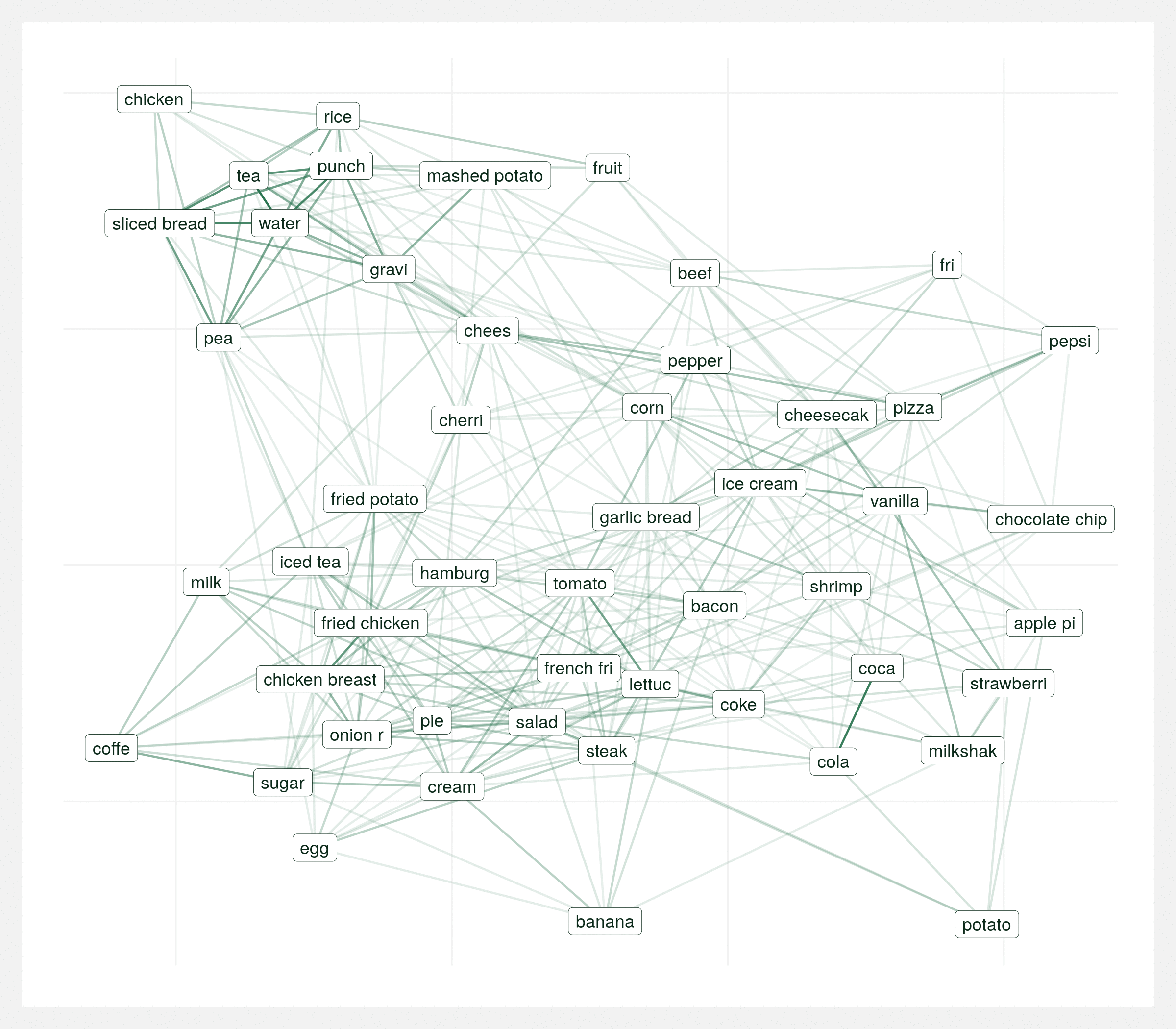
There are two clear communities. In the top-left section, simple comfort food such as mashed potatoes, gravy, tea, peas, and rice all naturally go together. In the center-right section, indulgent food such as hamburger, onion rings, fried chicken, and steak are grouped. Intuitively, cheese is stuck right in the middle of these two groups. I interpret this as it’s the great equalizer, almost everyone loves cheese and it goes with almost any food.
It’s important to view this graph a few different times with various random seeds. There’s many correct ways to visualize the same graph and sometimes you can draw the wrong conclusions from a single visualization so it’s important to take the above conclusions with some reservation. The below animation is the same data plotted 20 times with different seeds. Each plot varies but over the series of plots there’s still two consistent clusters.
Regional differences
I wanted to explore regional groupings but the data is much too skewed towards the South so any conclusions would be biased. It would be interesting to see if, for example, do southerners really enjoy home style more than others? Do midwesterners prefer corn? In lieu, we can do a simple count of the top items from each region. Note that the region is the region is which the execution occurred, not necessarily where the person was born.

Brands
It wouldn’t be American to not comment on brands within a capital punishment blog post. There’s surprisingly many. Coke takes the top spot overall and Kentucky Fried Chicken takes the top food spot. I guess you don’t have to worry about the side-effects of eating poorly, although one condemned prisoner did request antacids with their meal.

Final thoughts
The results are much cleaner than I expected with good separation in the cosine similarity graphs. The most difficult part of the analysis was working through the deduping steps. It was obvious from the beginning that uni-, bi-, and tr-grams were going to be needed along with somehow determining what was a food item vs. not. Removing stop words is simple but pulling coffee out of the string cup of coffee required tracking down a database of food and drinks.
The most difficult part was removing duplicates like the butter pecan ice cream example. We needed to extract ice cream even though butter pecan ice cream is within our list of food words. The key was to tokenize the data, filter for food words, group by the meal, and then search within the tokens for duplicates on a group-basis. A second iteration of this project should go one step further and try to separate pecans, hamburger, and butter pecan ice cream. You would want to extract pecans, hamburger, and ice cream. I think this could be accomplished with clever sequencing of tokenizing, filtering for food words, and doing recursive searches within the string. Although, a less rule-heavy approach may ultimately be best.
Packages used
library(tidyverse)
library(httr)
library(stringdist)
library(rvest)
library(stringr)
library(tidytext)
library(SnowballC)
library(igraph)
library(ggraph)
2020 February
Find the code here: github.com/joemarlo/Last-meals