Random forest from first principles
A bottom-up tutorial
This is a step-by-step guide to build a random forest classification algorithm in base R from the bottom-up. We will start with the Gini impurity metric then move to decision trees and then ensemble methods. The guide assumes basic statistics knowledge and medium familarity with R including functions and mapping.
R has many packages that include – faster and more flexible – implementations of random forest. The goal of this guide is to walk through the fundamentals. The final algorithm will be functional but it is not robust to bugs or programming edge cases. The goal is to provide you with an accurate mental model of how random forest works and, therefore, intuition to where it will perform well and where it falls short.
Process
Random forests are an ensemble model consisting of many decision trees. We will start at the lowest building block of the decision trees – the impurity metric – and build up from there. The steps to build a random forest are:
- Define an impurity metric which drives each split in the decision tree
- Program a decision algorithm to choose the best data split based on the impurity measure
- Program a decision tree algorithm by recursively calling the decision algorithm
- Program a bagging model by implementing many decision trees and resampling the data
- Program a random forest model by implementing many decision trees, resampling the data, and sampling from the columns
Intuition
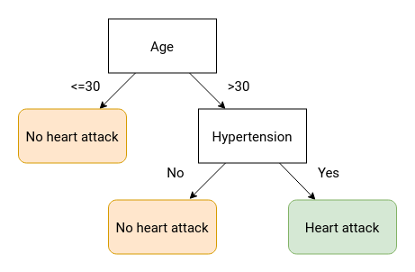
Binary decision trees create an interpretable decision-making framework for making a single prediction. Suppose a patient comes into your clinic with chest pain and you wish to diagnose them with either a heart attack or not a heart attack. A simple framework of coming to that diagnosis could look like the below diagram. Note that each split results in two outcomes (binary) and every possible condition leads to a terminal node.
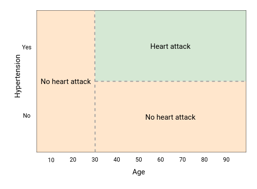
The model’s splits can also be visualized as partitioning the feature space. Since the decision tree makes binary splits along a feature, the resulting boundaries will always be rectangular. Further growing of the above decision tree will result in more but smaller boxes. Additional features (X1, X2, ...) will result in additional dimensions to the plot.
But where to split the data? The splits are determined via an impurity index. With each split, the algorithm maximizes the purity of the resulting data. If a potential split results in classes [HA, HA] and [NHA, NHA] then that is chosen over another split that results in [HA, NHA] and [NHA, HA]. At each node, all possible splits are tested and the split that maximizes purity is chosen.
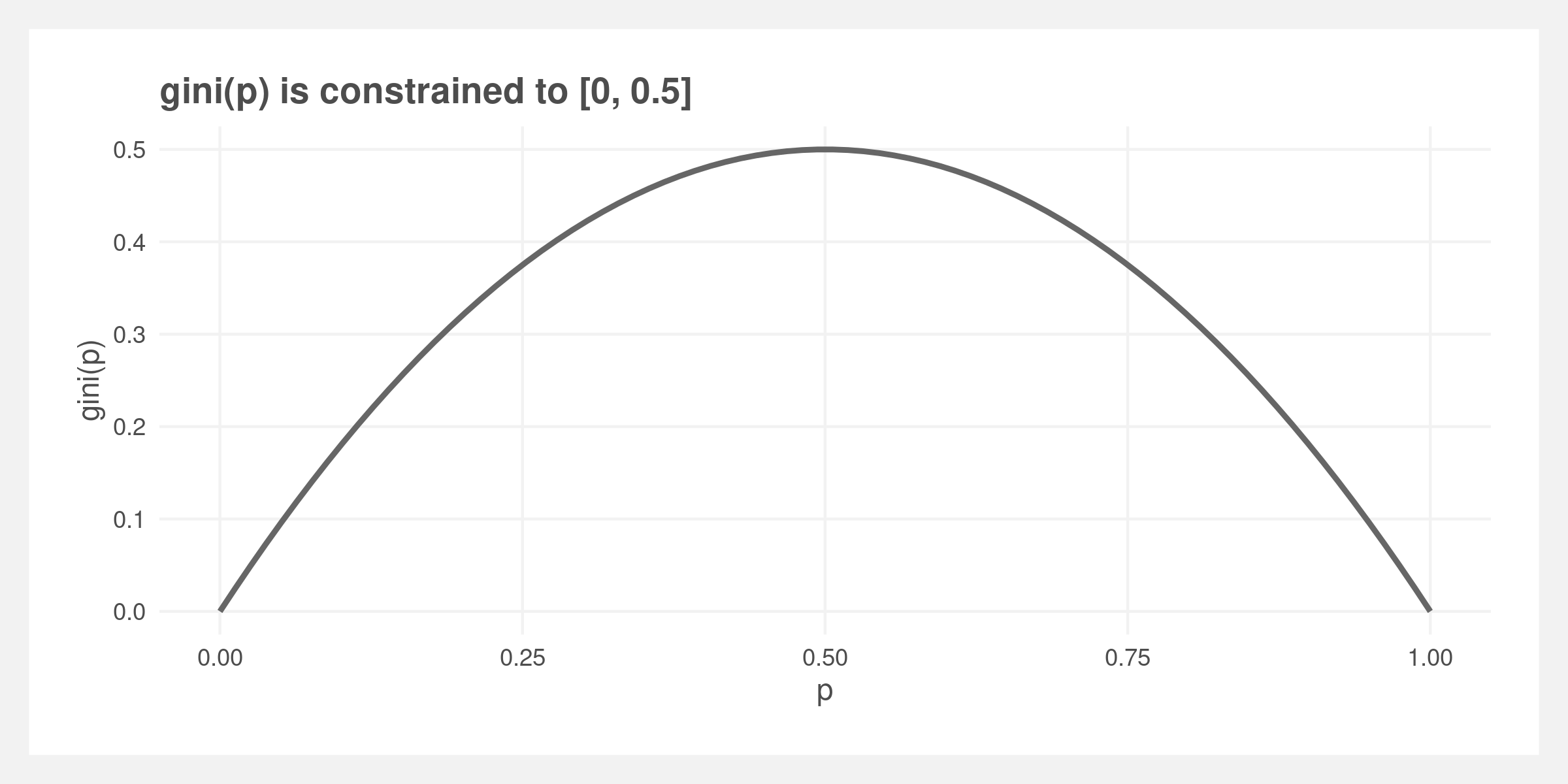
For classification problems, a commonly used metric is Gini impurity. Gini impurity is 2 * p * (1 - p) where p is the fraction of elements labeled as the class of interest. A value of 0 is a completely homogeneous vector while 0.5 is the inverse. The vector [NHA, HA, NHA] has a Gini value of 2 * 1/3 * 2/3 = 0.444. Since Gini is used for comparing splits, a Gini value is calculated per each resulting vector and then averaged – weighted by the respective lengths of the two vectors.
Setup
Okay, it’s not quite “base” R as we’re going to use the tidyverse meta-package for general data munging and parallel for multi-core processing during bagging and the random forest.
library(tidyverse)
library(parallel)
options(mc.cores = detectCores())
set.seed(44)
Gini impurity
We’re going to build the random forest algorithm starting with the smallest component: the Gini impurity metric. Note that the output of gini is constrained to [0, 0.5].
gini <- function(p) 2 * p * (1 - p)
For convenience, I am going to wrap the gini function so we feed it a vector instead of a probability. The probability is calculated from the mean value of the vector. In practice, this vector will be binary and represent classification labels so the mean value is the proportion of labels that represent a positive classification.
gini_vector <- function(X){
  # X should be binary 0 1 or TRUE/FALSE
  gini(mean(X, na.rm = TRUE))
}
X1 <- c(0, 1, 0)
gini_vector(X1)
## [1] 0.4444444
And finally I am going to wrap it again so it gives us the weighted Gini of two vectors.
gini_weighted <- function(X1, X2){
  # X should be binary 0 1 or TRUE/FALSE
  if (is.null(X1)) return(gini_vector(X2))
  if (is.null(X2)) return(gini_vector(X1))

  prop_x1 <- length(X1) / (length(X1) + length(X2))
  weighted_gini <- (prop_x1*gini_vector(X1)) + ((1-prop_x1)*gini_vector(X2))
  return(weighted_gini)
}
X2 <- c(1, 1, 1)
gini_weighted(X1, X2)
## [1] 0.2222222
Splitting
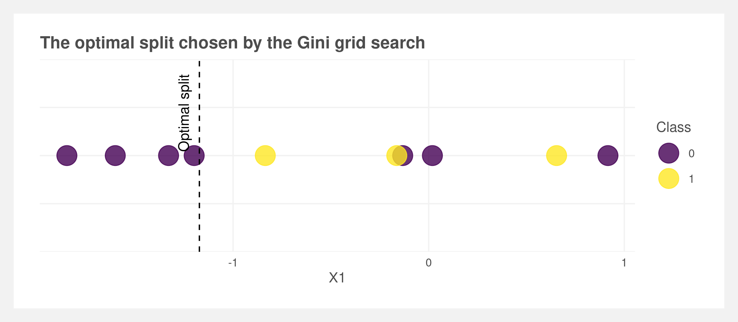
At each node, the tree needs to make a decision using the Gini metric. Here a single-dimensional grid search is performed to find the optimal value of the split for a given feature such as X1. Note that in formal packages like ranger this step is likely not a straight grid search and is optimized.
optimal_split <- function(X, classes, n_splits = 50){

  # create "dividing lines" that split X into to parts
  # a smarter version would account for X's values
  splits <- seq(min(X), max(X), length.out = n_splits)

  # calculate gini for each potential split
  gini_index <- sapply(splits, function(split){
    X1 <- classes[X <= split]
    X2 <- classes[X > split]
    gini_index <- gini_weighted(X1, X2)
    return(gini_index)
  })

  # choose the best split based on the minimum (most pure) gini value
  gini_minimum <- min(gini_index, na.rm = TRUE)
  optimal_split <- na.omit(splits[gini_index == gini_minimum])[1]

  # best prediction for these data are the means of the classes
  classes_split <- split(classes, X <= optimal_split)
  split0 <- tryCatch(mean(classes_split[[2]], na.rm = TRUE), error = function(e) NULL)
  split1 <- tryCatch(mean(classes_split[[1]], na.rm = TRUE),  error = function(e) NULL)
  preds <- list(split0 = split0, split1 = split1)

  return(list(gini = gini_minimum, split_value = optimal_split, preds = preds))
}
X <- rnorm(10)
classes <- rbinom(10, 1, 0.5)
optimal_split(X, classes)
## $gini
## [1] 0.3
##
## $split_value
## [1] -1.172117
##
## $preds
## $preds$split0
## [1] 0
##
## $preds$split1
## [1] 0.5
The grid search needs to be expanded to search all possible features (X1, X2, ...). The resulting smallest Gini value is the split the tree uses.
best_feature_to_split <- function(X, Y){
  # X must be a dataframe, Y a vector of 0:1

  # get optimal split for each column
  ginis <- sapply(X, function(x) optimal_split(x, Y))

  # return the the column with best split and its splitting value
  best_gini <- min(unlist(ginis['gini',]))[1]
  best_column <- names(which.min(ginis['gini',]))[1]
  best_split <- ginis[['split_value', best_column]]
  pred <- ginis[['preds', best_column]]
  return(list(column = best_column, gini = best_gini, split = best_split, pred = pred))
}
n <- 1000
.data <- tibble(Y = rbinom(n, 1, prob = 0.3),
                X1 = rnorm(n),
                X2 = rnorm(n),
                X3 = rbinom(n, 1, prob = 0.5))
X <- .data[, -1]
Y <- .data[[1]]
best_feature_to_split(.data[, -1], .data[['Y']])
## $column
## [1] "X1"
##
## $gini
## [1] 0.4046333
##
## $split
## [1] -2.726038
##
## $pred
## $pred$split0
## [1] 1
##
## $pred$split1
## [1] 0.2825651
Decision trees
Recursion
To create the decision trees, the splitting algorithm should be applied until it reaches a certain stopping threshold. It is not known prior how many splits it is going to make – the depth or the width. This is not easily solved using a while loop as a split results in two new branches and each can potentially split again. Recursion is required.
In recursive functions, the function is called within itself until some stopping criteria is met. A simple example is the quicksort algorithm which sorts a vector of numbers from smallest to greatest.
Quicksort is a divide-and-conquer method that splits the input vector into two vectors based on a pivot point. Points smaller than the pivot go to one vector, points larger to the other vector. The pivot point can be any point but is often the first or last item in the vector. The function is called on itself to repeat the splitting until one or less numbers exist in the resulting vector. Then these sorted child-vectors are passed upward through the recursed functions and combined back into a single vector that is now sorted.
quick_sort <- function(X){

  # stopping criteria: stop if X is length 1 or less
  if (length(X) <= 1) return(X)

  # create the pivot point and remove it from the vector
  pivot_point <- X[1]
  X_vec <- X[-1]

  # create the lower and upper vectors
  lower_vec <- X_vec[X_vec <= pivot_point]
  upper_vec <- X_vec[X_vec > pivot_point]

  # call the function recursively
  lower_sorted <- quick_sort(lower_vec)
  upper_sorted <- quick_sort(upper_vec)

  # return the sorted vector
  X_sorted <- c(lower_sorted, pivot_point, upper_sorted)
  return(X_sorted)
}
X <- rnorm(20)
quick_sort(X)
##  [1] -1.288492187 -1.012602888 -0.938064465 -0.815872056 -0.495430743
##  [6] -0.479283544 -0.477149902 -0.445188837 -0.008493793  0.112405152
## [11]  0.176615746  0.389688918  0.454000688  0.507450697  0.615812243
## [16]  0.947849356  1.415313533  1.423378109  1.457175891  1.813671874
Recursive branching
We’re going to implement the above splitting algorithm as a recursive function which builds our decision tree classifier. The tree will stop if it exceeds a certain depth, a minimum number of observations result from a given split, or if the Gini measure falls below a certain amount. Only one of these methods is required however including all three allow additional hyperparameter tuning down-the-road.
The function recursively calls the best_feature_to_split() function until one of the stopping criteria is met. All other code is to manage the saving of the split decisions. The output is a dataframe denoting these decisions. The m_features argument denotes the number of columns to be used at each split – this will be useful later for random forest.
# create a dataframe denoting the best splits
decision_tree_classifier <- function(X, Y, gini_threshold = 0.4, max_depth = 5, min_observations = 5, branch_id = '0', splits = NULL, m_features = ncol(X)){

  # sample the columns -- for use later in random forest
  m_features_clean <- min(ncol(X), max(2, m_features))
  sampled_cols <- sample(1:ncol(X), size = m_features_clean, replace = FALSE)
  X_sampled <- X[, sampled_cols]

  # calculate the first optimal split
  first_split <- best_feature_to_split(X_sampled, Y)

  # save the splits
  if (is.null(splits)) splits <- tibble()
  splits <- bind_rows(splits, tibble(column = first_split$column,
                                     split = first_split$split,
                                     pred = list(first_split$pred),
                                     branch = branch_id))

  # create two dataframes based on the first split
  X_split <- split(X, X[first_split$column] >= first_split$split)
  Y_split <- split(Y, X[first_split$column] >= first_split$split)

  # check if stopping criteria is met
  is_too_deep <- isTRUE(nchar(branch_id) >= max_depth)
  is_pure_enough <- isTRUE(first_split$gini <= gini_threshold)
  too_few_observations <- isTRUE(min(sapply(X_split, nrow)) < min_observations)

  # stop here if criteria is met
  if (is_too_deep | is_pure_enough | too_few_observations) return(splits)

  # otherwise continue splitting
  # the try will catch errors due to one split group having no observations
  split0 <- tryCatch({
    decision_tree_classifier(
      X = X_split[[1]],
      Y = Y_split[[1]],
      gini_threshold = gini_threshold,
      max_depth = max_depth,
      min_observations = min_observations,
      branch_id = paste0(branch_id, "0"),
      splits = splits,
      m_features = m_features
    )
  }, error = function(e) NULL
  )
  split1 <- tryCatch({
    decision_tree_classifier(
      X = X_split[[2]],
      Y = Y_split[[2]],
      gini_threshold = gini_threshold,
      max_depth = max_depth,
      min_observations = min_observations,
      branch_id = paste0(branch_id, "1"),
      splits = splits,
      m_features = m_features
    )
  }, error = function(e) NULL
  )

  # bind rows into a dataframe and remove duplicates caused by diverging branches
  all_splits <- distinct(bind_rows(split0, split1))

  return(all_splits)
}
# test the function
n <- 1000
.data <- tibble(Y = rbinom(n, 1, prob = 0.3),
                X1 = rnorm(n),
                X2 = rnorm(n),
                X3 = rbinom(n, 1, prob = 0.5))
X <- .data[, -1]
Y <- .data[[1]]
decision_tree <- decision_tree_classifier(X, Y, 0.1)
decision_tree
## # A tibble: 17 x 4
##    column   split pred             branch
##    <chr>    <dbl> <list>           <chr>
##  1 X2     -1.22   <named list [2]> 0
##  2 X2     -1.26   <named list [2]> 00
##  3 X1      1.99   <named list [2]> 000
##  4 X2     -1.23   <named list [2]> 001
##  5 X1     -1.52   <named list [2]> 01
##  6 X2      0.149  <named list [2]> 010
##  7 X1     -1.77   <named list [2]> 0100
##  8 X2      0.0631 <named list [2]> 01000
##  9 X1     -1.62   <named list [2]> 01001
## 10 X1     -1.56   <named list [2]> 0101
## 11 X2      0.110  <named list [2]> 011
## 12 X2     -0.117  <named list [2]> 0110
## 13 X2     -0.165  <named list [2]> 01100
## 14 X2      0.0502 <named list [2]> 01101
## 15 X2      0.478  <named list [2]> 0111
## 16 X1      1.06   <named list [2]> 01110
## 17 X2      0.586  <named list [2]> 01111
And that is all there is to a decision tree classifier – just a recursive algorithm that splits the data based on some purity metric.
Predictions
A new observation is predicted by traversing the decision tree model via recursion. For a given point, start at branch_id = 0, calculate if the value is above or below the split, and then go “left” or “right” by appending the branch_id with a 0 or 1. Repeat until there are no branches left.
# predict a new data point
predict_data_point <- function(model_decision_tree, new_row, branch_id = '0'){

  # traverse the decision tree and get the next split
  decision_point <- model_decision_tree[model_decision_tree$branch == branch_id,]
  decision_split <- new_row[, decision_point$column] < decision_point$split
  decision_split <- if_else(decision_split, 0, 1)
  branch_id <- paste0(branch_id, decision_split)

  # if the new branch_id (i.e. the next split) is not in the decision tree then return the current prediction
  if (!(branch_id %in% model_decision_tree$branch)){
    pred <- decision_point$pred[[1]][[decision_split + 1]]
    return(pred)
  }

  # otherwise continue recursion
  return(predict_data_point(model_decision_tree, new_row, branch_id))
}
predict_data_point(decision_tree, X[1,])
## [1] 0.3252033
Wrap the predict_data_point function in a loop so it can predict all observations in a dataframe.
# predict all datapoints in a dataframe
predict_decision_tree <- function(model_decision_tree, new_data){
  preds <- rep(NULL, nrow(new_data))
  for (i in 1:nrow(new_data)){
    preds[i] <- predict_data_point(model_decision_tree, new_row = new_data[i,])
  }
  return(preds)
}
preds <- predict_decision_tree(decision_tree, X)
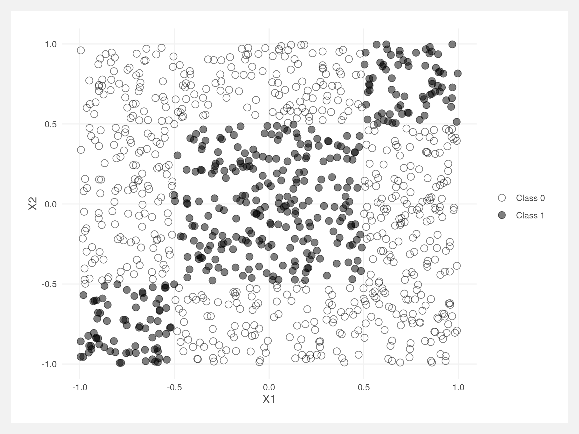
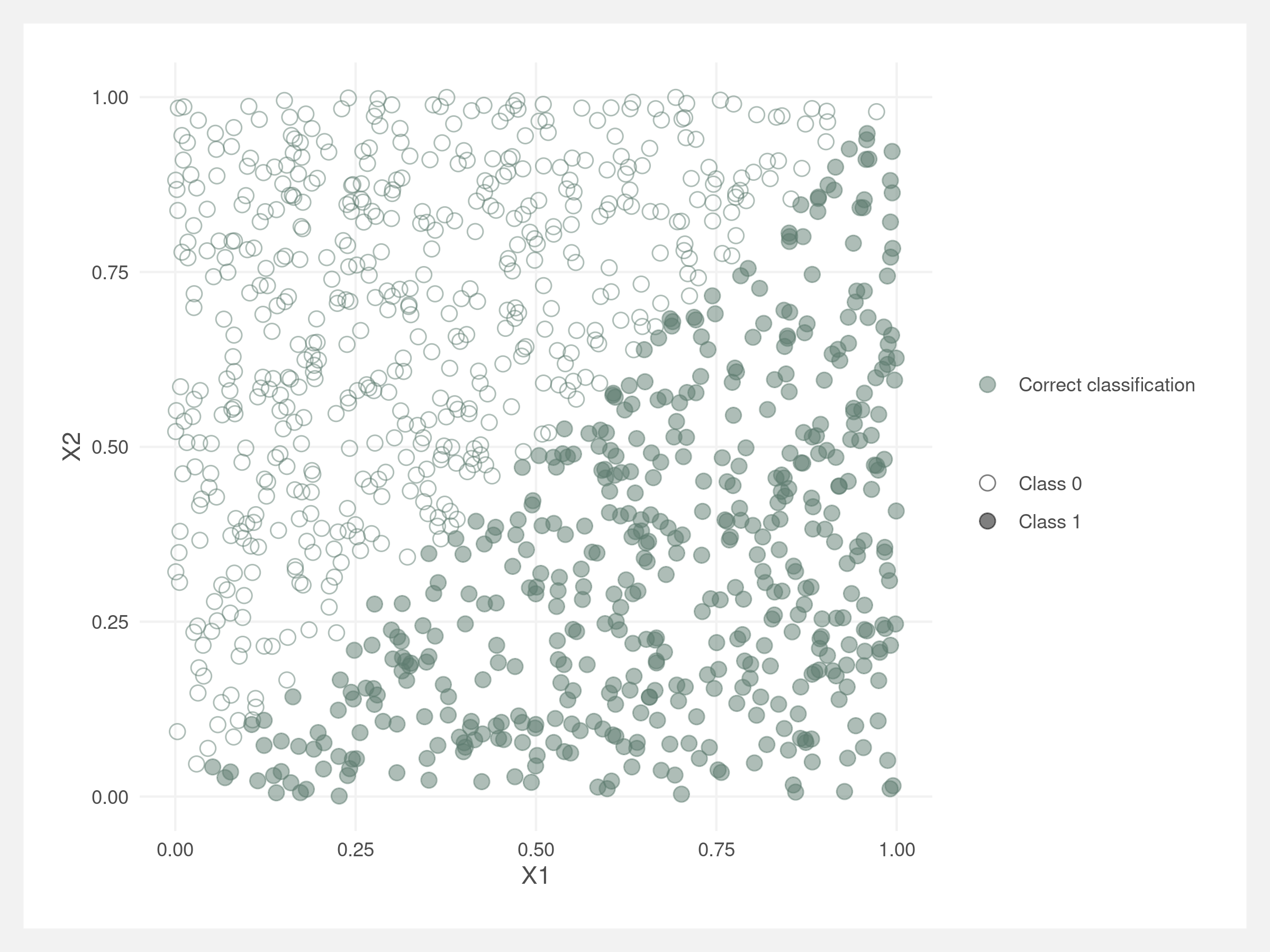
Finally, we can test our decision tree classifier on data. Decision trees perform best on data split horizontally and/or vertically – i.e. on data where linear regression or logistic regression tends to perform poorly. Here I create “boxed” data where the boxes delineate between Class 0 and Class 1.
# create a two dimensional dataset
n <- 1000
.data <- tibble(X1 = runif(n, -1, 1),
                X2 = runif(n, -1, 1),
                Y = (round(X1) == round(X2)) * 1)
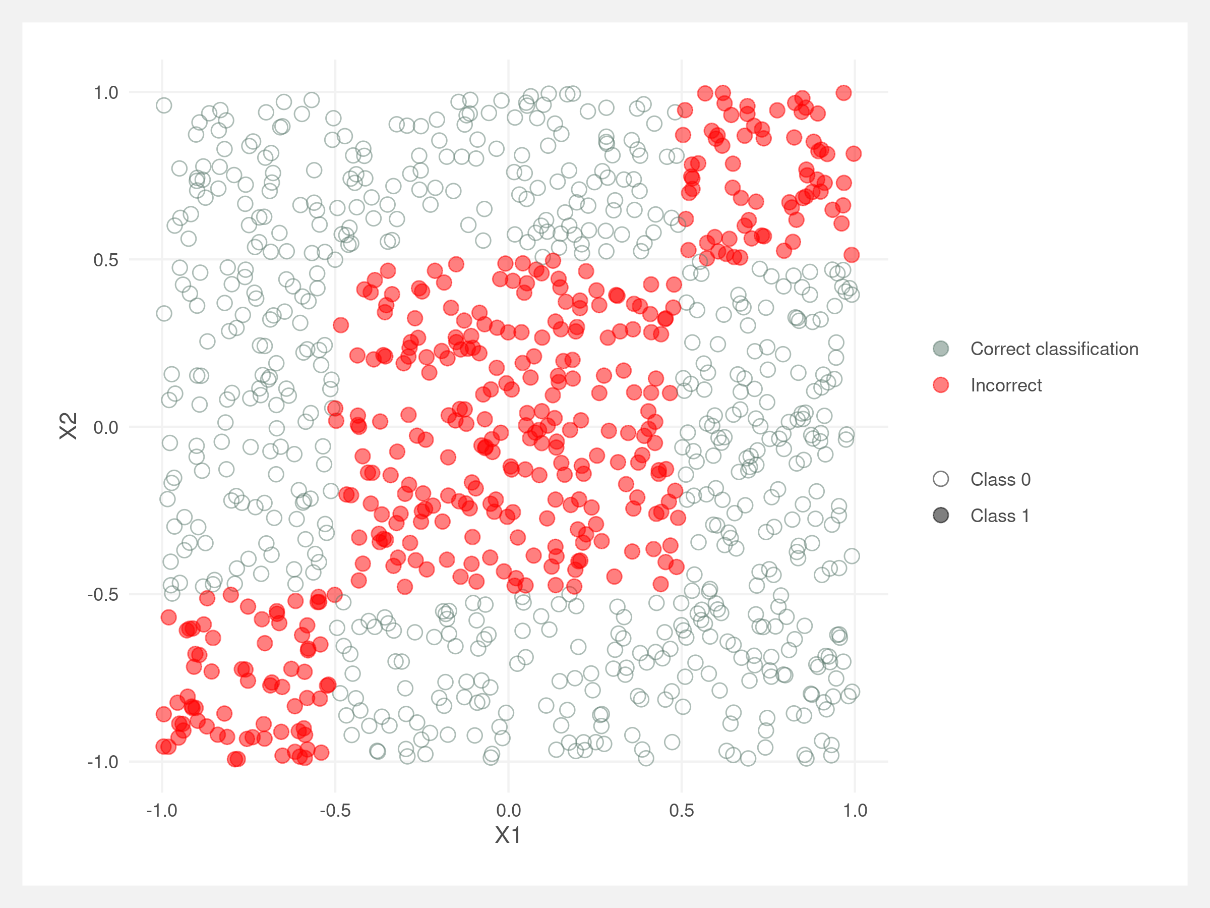
Classifying these points with a logistic regression results in poor performance. The red indicates misclassified points.
# logistic regression
model_log <- glm(Y ~ X1 + X2, data = .data, family = 'binomial')
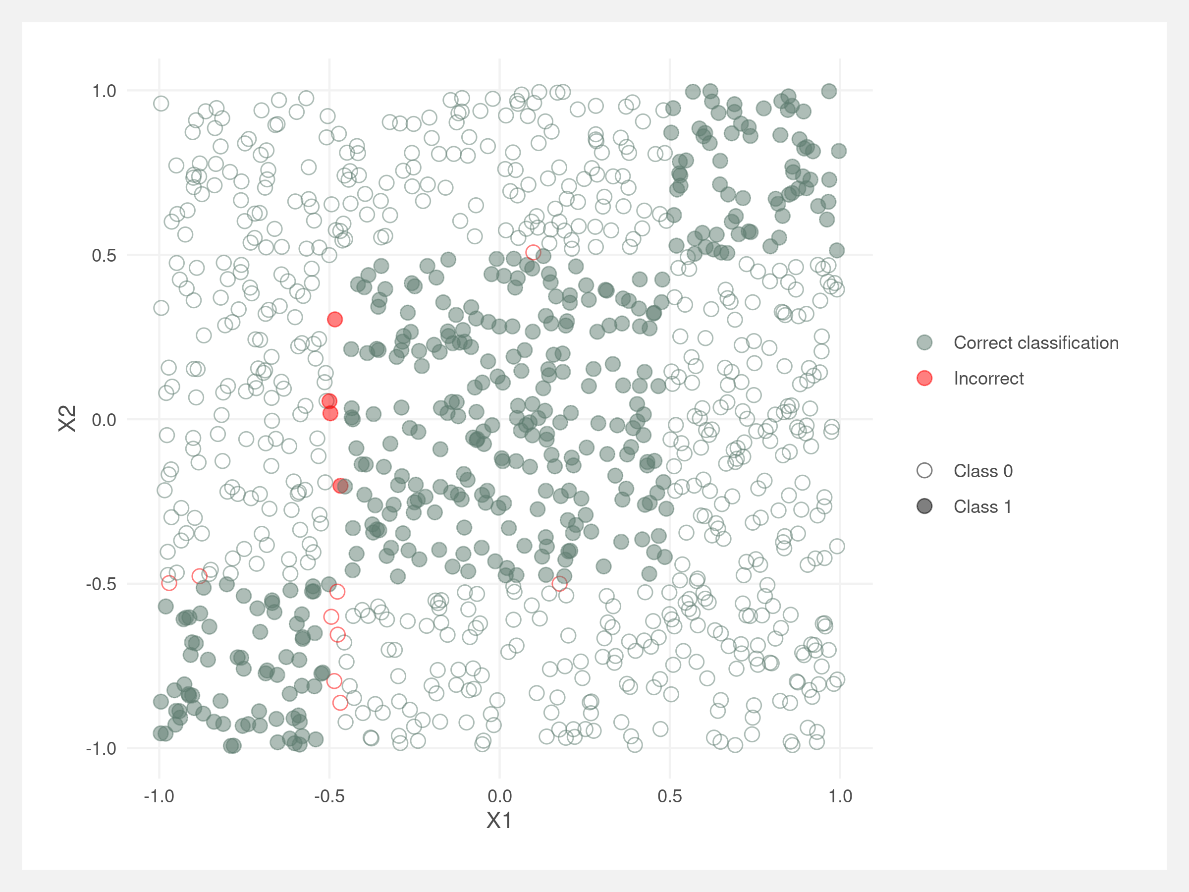
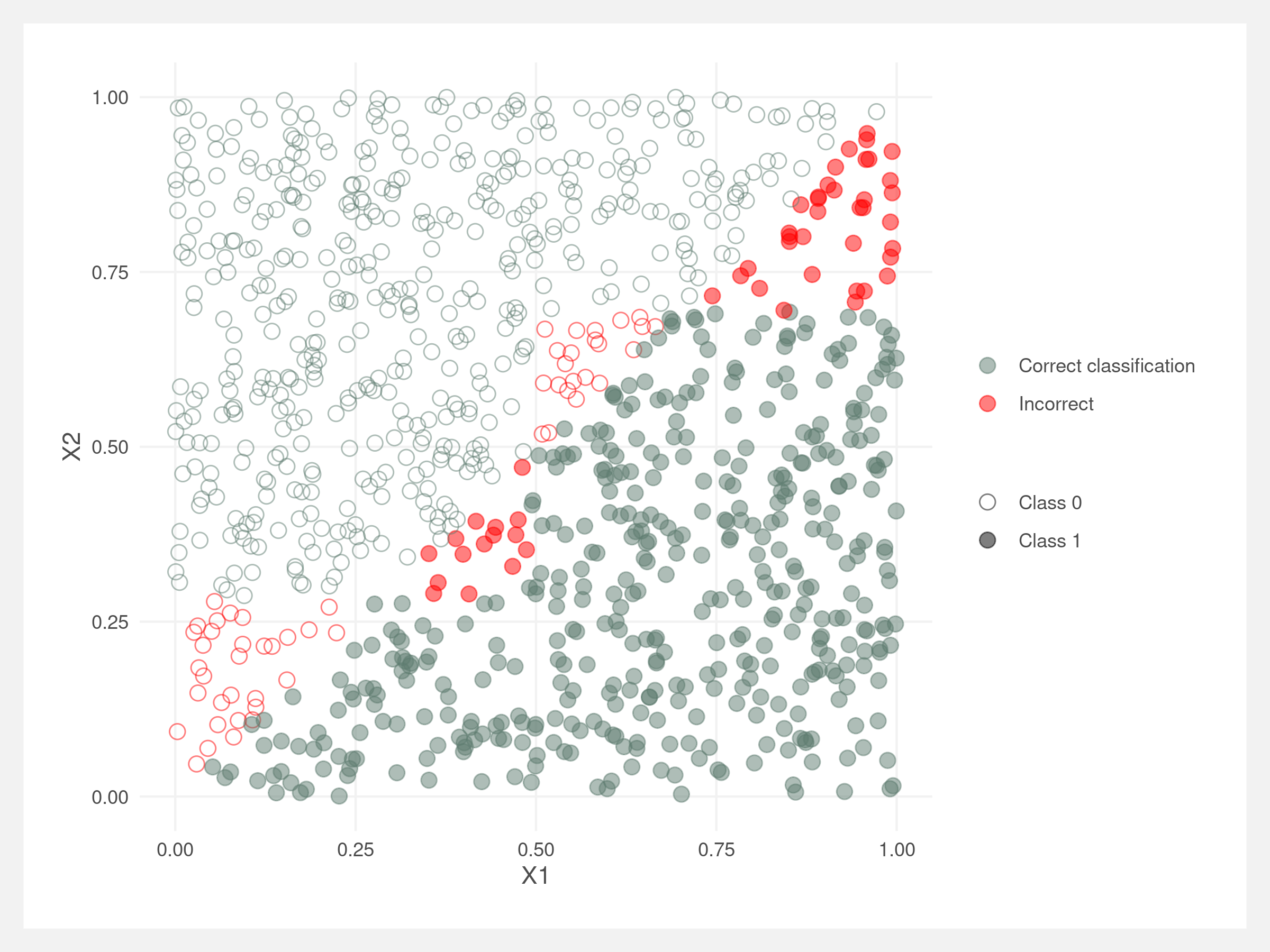
These “square” data suit the decision tree classifier well. Below, the classifier correctly classifies almost all points. The incorrect points all lie around the boundary between Class 0 and Class 1. This may be due to the splits in optimal_split() not being granular enough.
X <- dplyr::select(.data, -Y)
Y <- .data[['Y']]
model_decision_tree <- decision_tree_classifier(X, Y, max_depth = 4,
						gini_threshold = 0,
						min_observations = 1)
preds <- predict_decision_tree(model_decision_tree, X)
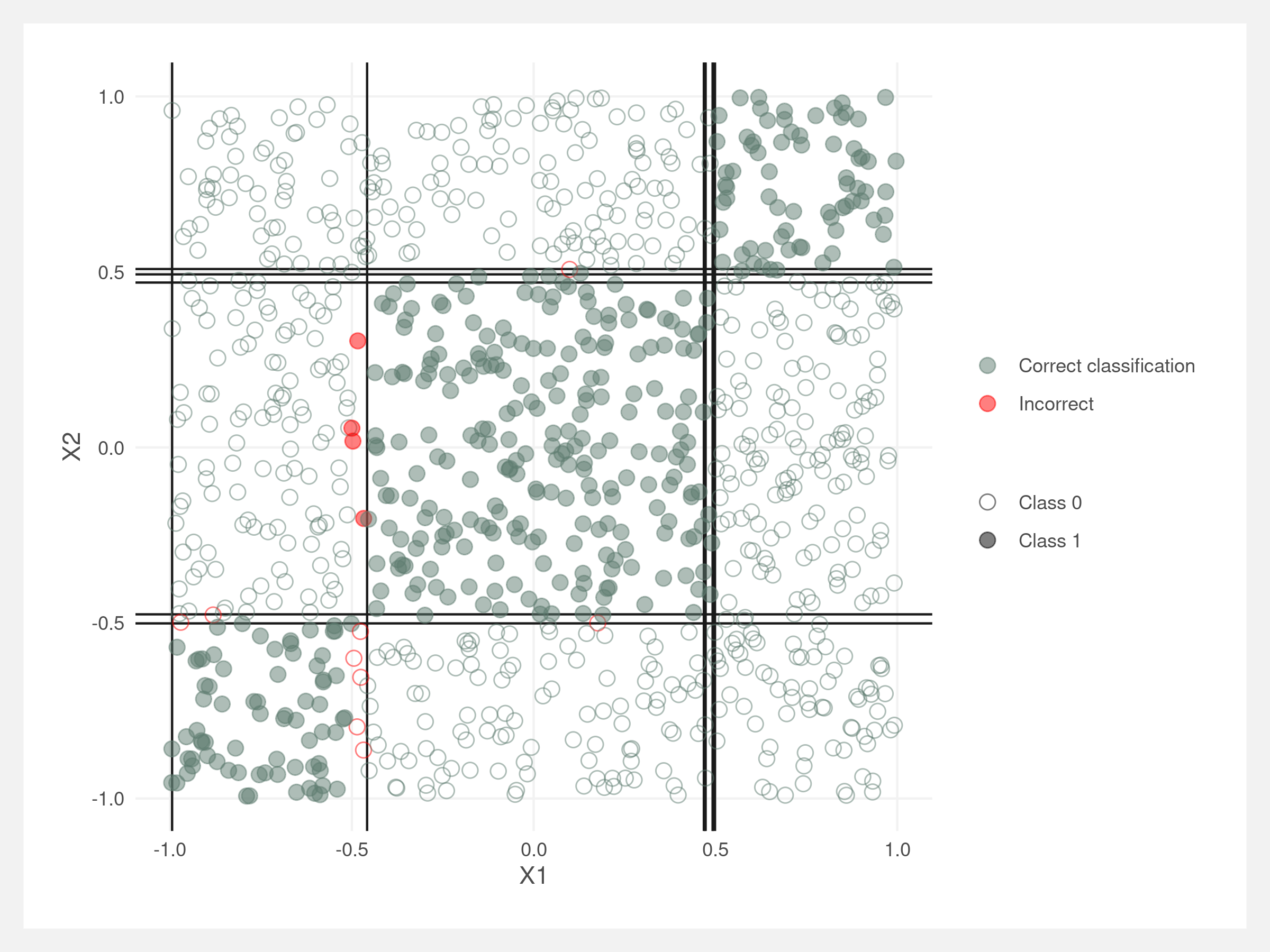
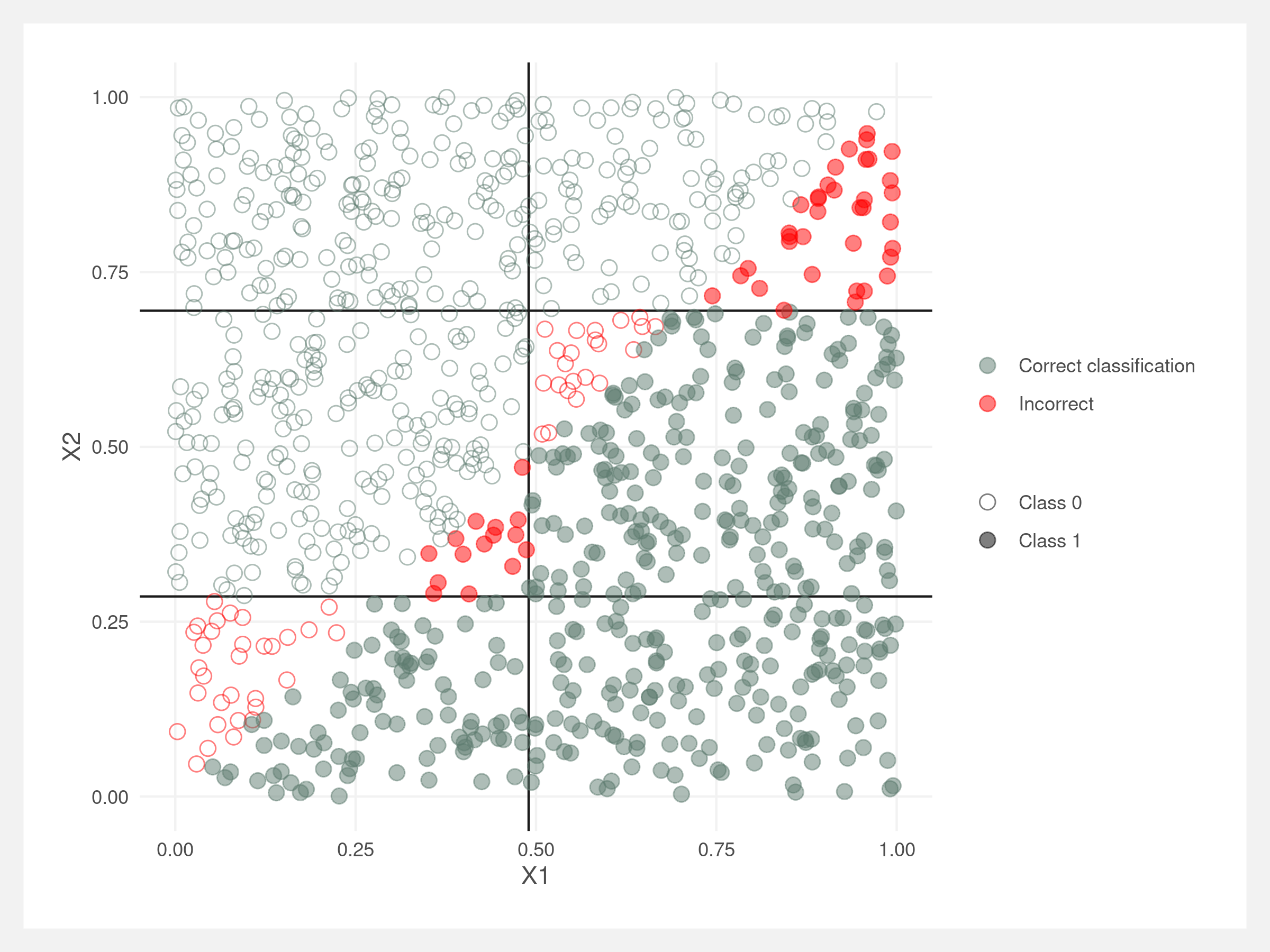
We can visualize the splits made by the decision tree classifier. They should be right along the rectangle boundaries. Note that these lines do not account for the order of the splits – the lines would need to be truncated at their parent node’s line, similar to the diagram in the introduction.
Where trees struggle
Trees will struggle when the feature space is dissected at an angle by the classification value. Since decision trees are partitioning the feature space into rectangles, the tree will need to be deeper to approximate the decision boundary.
The below data’s classification is in two separate triangles: top left and bottom right of the plot. A logistic regression finds the boundary easily.
A decision tree has a difficult time finding the decision boundary.
The decision tree’s rectangles are not enough to approximate the angled boundary.
Bagging
Single decision trees are prone to overfitting and can have high variance on new data. A simple solution is to create many decision trees based on resamples of the data and allow each tree to “vote” on the final classification. This is bagging. The process keeps the low-bias of the single tree model but reduces overall variance.
The “vote” from each tree is their prediction for a given observation. The votes are averaged across all the trees and the final classification is determined from this average. The trees are trained on bootstrapped data – taking repeated samples of the training data with replacement.
bag_it <- function(X_train, Y_train, X_test, n_trees = 100, max_depth = 5, gini_threshold = 0.2, min_observations = 5){

  # grow the trees
  preds <- parallel::mclapply(1:n_trees, function(i){

    preds <- tryCatch({

      # bootstrap the data
      sample_indices <- sample(1:nrow(X_train), size = nrow(X_train), replace = TRUE)
      X_sampled <- X_train[sample_indices,]
      Y_sampled <- Y_train[sample_indices]

      # fit model on subset and then make predictions on all data
      model_decision_tree <- decision_tree_classifier(X_sampled, Y_sampled,
      						      max_depth = max_depth,
      						      gini_threshold = gini_threshold,
      						      min_observations = min_observations)
      preds <- predict_decision_tree(model_decision_tree, X_test)
    },
    error = function(e) NA
    )

    return(tibble(preds))
  }) %>% bind_cols()

  # average the predictions across each model's prediction
  # this is how each tree "votes"
  preds <- rowMeans(preds, na.rm = TRUE)
  return(preds)
}
# read in the credit data
credit <- read_csv(file.path(wd, "data/credit_card.csv"))
X <- select(credit, -Class)
Y <- credit$Class

# create train test split
indices <- sample(c(TRUE, FALSE), size = nrow(credit), replace = TRUE, prob = c(0.5, 0.5))
X_train <- X[indices,]
X_test <- X[!indices,]
Y_train <- Y[indices]
Y_test <- Y[!indices]
# fit the bagged model
preds <- bag_it(X_train, Y_train, X_test, n_trees = 50, max_depth = 10,
		gini_threshold = 0, min_observations = 5)
table(preds > 0.5, Y_test)
##        Y_test
##           0   1
##   FALSE 485  33
##   TRUE    9 221
Random forest
Random forest is like bagging except in addition to bootstrapping the observations, you also take a random subset of the features at each split. The rule-of-thumb sample size is the square root of the total number of features. We’ll implement this by utilizing the optional m_features argument we added earlier to decision_tree_classifier().
random_forest <- function(X_train, Y_train, X_test, n_trees = 100, m_features = ceiling(sqrt(ncol(X_train))), max_depth = 5, gini_threshold = 0.2, min_observations = 5){

  # grow the trees
  preds <- parallel::mclapply(1:n_trees, function(i){

    preds <- tryCatch({

      # bootstrap the data
      sample_indices <- sample(1:nrow(X_train), size = nrow(X_train), replace = TRUE)
      X_sampled <- X_train[sample_indices,]
      Y_sampled <- Y_train[sample_indices]

      # fit model on subset and then make predictions on all data
      model_decision_tree <- decision_tree_classifier(
        X_sampled,
        Y_sampled,
        max_depth = max_depth,
        gini_threshold = gini_threshold,
        min_observations = min_observations,
        m_features = m_features
      )
      preds <- predict_decision_tree(model_decision_tree, X_test)
    },
    error = function(e) NA
    )

    return(tibble(preds))
  }) %>% bind_cols()

  # average the predictions across each model's prediction
  # this is how each tree "votes"
  preds <- rowMeans(preds, na.rm = TRUE)
  return(preds)
}
# fit the random forest
preds <- random_forest(X_train, Y_train, X_test, n_trees = 50, max_depth = 10,
		       gini_threshold = 0, min_observations = 5)
table(preds > 0.5, Y_test)
##        Y_test
##           0   1
##   FALSE 487  32
##   TRUE    7 222
Compare this against the ranger package’s random forest algorithm.
model_ranger <- ranger::ranger(Class ~ ., data = credit[indices,], num.trees = 50, max.depth = 10)
preds <- predict(model_ranger, data = credit[!indices,])$predictions
table(preds > 0.5, credit$Class[!indices])
##           0   1
##   FALSE 481  29
##   TRUE   13 225
Not bad! Looks like our function performs just as well on this dataset as the formal ranger package.
Conclusion
Benefits of tree methods:
- Single trees are easy to explain and interpret
- Allows for both classification and regression
- For regression, replace the Gini impurity measure with variance of the outcome variable
- Allows for binary, continuous, and categorical (with dummy coding) variables
- Can handle missing data (if data is not used within a branch)
- Ensemble methods are computationally parallelizable
Downsides:
- Single trees are easy to overfit
- Single trees have high variance
- Ensemble methods are difficult to interpret
2021 April
Find the code here: github.com/joemarlo/regression-trees