Claiming Social Security benefits
Optimizing Social Security and market Monte Carlos
Why write about this?
- Social Security is the largest source of income for most American retirees
- Social Security is known as a great equalizer across races where there is savings inequality and reportedly a general retirement savings crisis
- Social Security is something Americans routinely mess up by claiming too early
Social Security is complicated. Luckily, there’s plenty written on how it works for the fastidious reader. Every eligible American should understand the very basics that directly impact their benefits check and the implicit tradeoffs they are making when they file to claim their benefits. I won’t dive into the specifics of how the claiming process works but you should know that you can claim as early as age 62 and you receive a permanent increase in benefits for each month you wait to claim until age 70.
This leads to the question:
At what age should I claim Social Security in order to receive the most amount of money?
Or more specifically:
At what age should I claim Social Security based on how long I expect to live and, if I invest the money, what rate of return I expect to earn in the market?
This is commonly asked by financial advisors who serve the wealthy, but perhaps less so by the individuals who make these financial decisions themselves. These advisors tend to assume it’s best to claim early, hand that money over to the advisor, and have them invest in the market (and reap the associated fees).
To answer the question, I’ve done the work to calculate all the various possible combinations of outcomes and presented it in the below plot. It describes the best age to claim Social Security while capturing the relationship between life expectancy (also known as longevity) and investment return. To use, pick a longevity and expected investment return, go to the intersection and the color indicates which claim age is best.
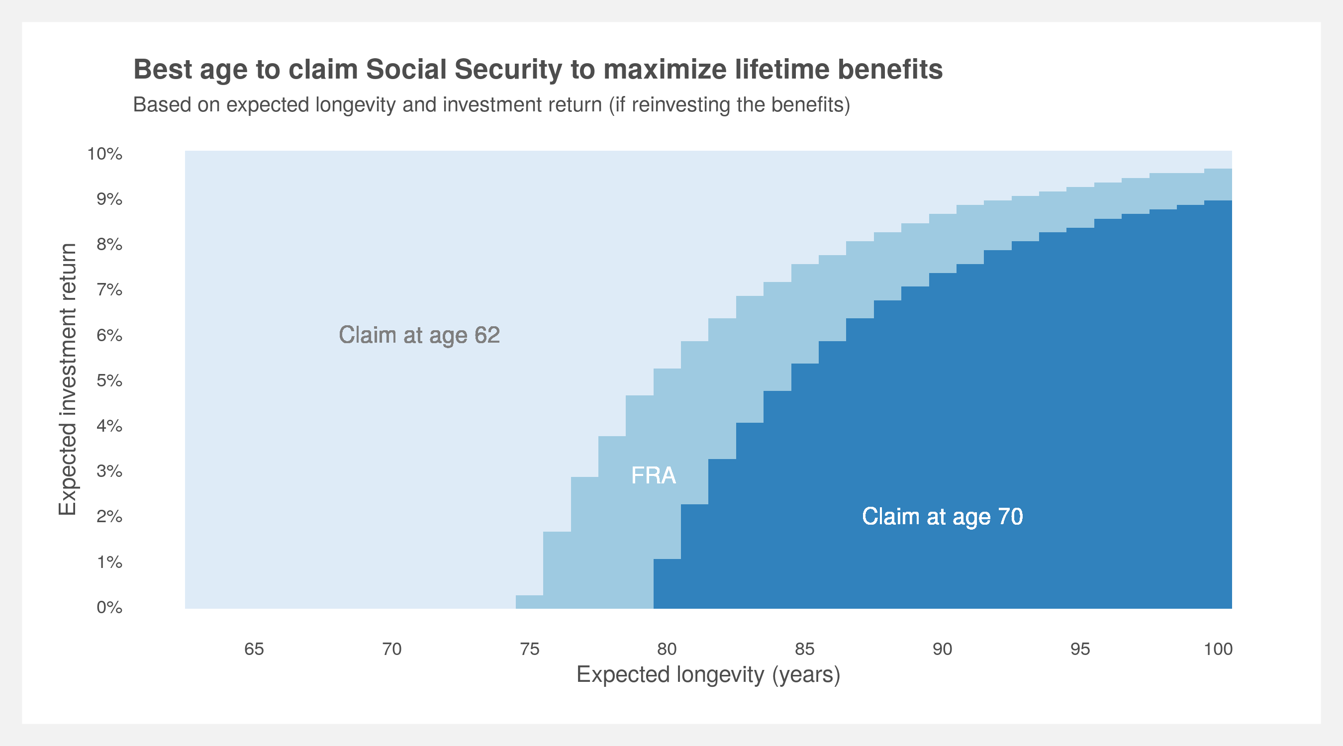
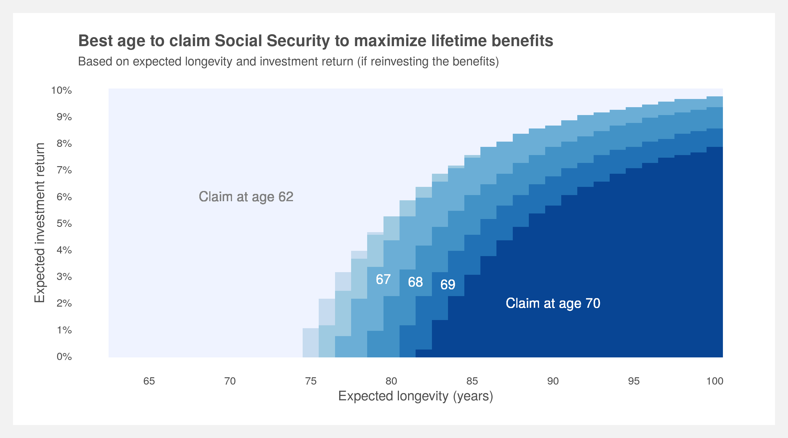
This is a simplified result with only three solutions: age 62, Full Retirement Age (FRA, ~66) and 70. A more comprehensive plot with all ages between 62 and 70 is presented in the How to build your own analysis section below.
Life expectancy may be hard to estimate for yourself but family member experience and life expectancy tables starting at age 62 are a good place to start. The decision between uncertain market return and guaranteed U.S. government money is much more tractable. If you want to learn more about long-term market expectations, you can find more here.
The plot tells us it’s always better to wait until 70 if you don’t plan on investing the benefits and believe you’ll live past 80. If you do plan on investing the benefits, at an investment return of 5% (probably a safe bet for most people) and using a life expectancy of age 90 (about average for a couple currently age 62), claiming at age 70 is still the best choice to maximize lifetime benefits. If you’re optimistic about the market and believe you can yield at least 9% consistently every year, feel free to claim as early as you wish. However, note that this is a trade-off between a guaranteed, government-backed increase and volatile market returns. More on market uncertainty below.
How to build your own analysis
If you’re interested in building and tweaking this model yourself, you can find all the code on my github. Here’s the basic structure of the analysis:
- First build a Social Security benefits calculator based on the laws, IRS code, and maybe recent legislation. Not as difficult as one would imagine if you know where to look
- Calculate Social Security benefits for a given claim age and life expectancy. “Invest” those benefits at some rate
- Discount those benefits back to age 62 at a rate equal to inflation. This is the present value of the benefits
- Repeat steps 2 & 3 for every combination of claim age, life expectancy, and investment return rate (this is a brute force method)
- Find the claim age that maximizes the present value for each combination of life expectancy and investment return rate
- Optional: simulate the rates to account for market uncertainty
The calculator
The calculator should return annual Social Security benefits and allow the user to tweak birth year, claim age, and wage history. Wages are capped at the applicable amount. The top 35 years of earnings are captured to calculate the Average Indexed Monthly Earnings and then the Primary Insurance Amount. Benefits are forecasted into the future based on expected Cost-of-Living-Adjustment. COLA itself is based on inflation, specifically CPI-W. Since individual Social Security benefits discontinue at time of death the benefits stop at the expected longevity of the person. The calculator can be tested against this calculator from the Social Security Administration.
You can find the calculator in R form here: SS_calculator.R.
Helper functions
Several helper functions need to be written to expedite the analysis. The functions need to perform the following:
- add investment return to a series of cash flows
- simulate investment return over a series of cash flows and then return a specified quantile value
- calculate present value and net present value (these can also be found in third-party packages)
You can find the helper functions in R form here: Helper_functions.R.
The discounting process
We can determine the value of a series of benefits by simple net present value (NPV) discounted at the rate of inflation. First, calculate the benefits using the benefits calculator then take the NPV.
# calculate the NPV of a series of annual benefits
benefits <- calculate_benefits(birth.year = 1957, claim.age = 62) %>% filter(Age >= 62)
NPV(benefits$Benefits, inflation.rate)
[1] 430684.4
Now, repeat this process for all the claim ages between 62 and 70 then plot it.
# plot of NPVs by claim age
sapply(62:70, function(claim.age){
  calculate_benefits(birth.year = 1957, claim.age = claim.age) %>%
    filter(Age >= 62) %>%
    pull(Benefits) %>%
    NPV(., inflation.rate)
}) %>%
  enframe() %>%
  ggplot(aes(x = name, y = value)) +
  geom_col(fill = '#2b7551') +
  scale_x_continuous(breaks = 1:9,
                     labels = 62:70) +
  scale_y_continuous(labels = scales::dollar_format()) +
  labs(title = "Net present value of SS benefits by claim age",
       x = "Claim age",
       y = "NPV of benefits") +
  light.theme
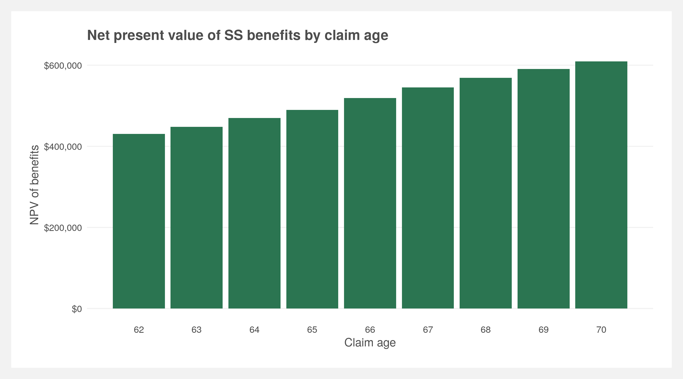
However, what we want to know is how much is a series of benefits worth if one invests their benefits and it yields a certain rate of return. We can treat the accumulation of benefits as an investment account with annual deposits and compounded growth at a given rate. Then we can take the terminal (final) value and discount it back to age 62. This will give us a single value that is an apples-to-apples comparison once we start varying the claim age.
# calculate the present value of one series of benefits, starting at age 62,
#  ending at age 100, and with an an investment return of 5%
benefits$Benefits %>%
  add_investment_return(., rate = 1.05) %>%
  last(.) %>%
  PV(., rate = inflation.rate, periods = 100-62)
[1] 706134
Great. Now let’s calculate this present value across various investment returns, claim ages, and longevities.
# set the investment returns, claim ages, and death ages we are interested in
inv.returns <- seq(1, 1.1, by = 0.001) # this is 0->10%
claim.ages <- 62:70
death.ages <- 63:100

# create all combinations of investment returns, claim age, and death age
PV.grid <- expand.grid(Return = inv.returns,
                       Claim.age = claim.ages,
                       Death.age = death.ages) %>% as_tibble()

# calculate PV for all the combinations
PV.grid$PV <-
  pmap(list(PV.grid$Return, PV.grid$Claim.age, PV.grid$Death.age),
       function(inv.return, age, death) {
         # calculate benefits then add investment return then calculate present value
         calculate_benefits(birth.year = 1957, claim.age = age) %>%
           filter(Age >= 62,
                  Age <= death) %>%
           pull(Benefits) %>%
           add_investment_return(., inv.return) %>%
           last(.) %>%
           PV(., rate = inflation.rate, periods = death - 62)

       }) %>% unlist()

head(PV.grid)
# A tibble: 6 x 4
  Return Claim.age Death.age     PV
   <dbl>     <int>     <int>  <dbl>
1   1           62        63 21867.
2   1.00        62        63 21878.
3   1.00        62        63 21889.
4   1.00        62        63 21900.
5   1.00        62        63 21910.
6   1.00        62        63 21921.
We now have present values for every combination of investment return, claim age, and longevity. What we really care about is the best claim age for a given investment return and longevity. To find this, we can take the maximum present value for a given grouping of investment return and longevity.
We can now build the plot shown at the beginning of the post. A simple table will do but that might miss the bigger pattern. This one will be bit more detailed as every age between between 62 and 70 was calculated, not just age 62, 66 (FRA), and 70.
# plot of best claim age by investment return and death age
PV.grid %>%
  group_by(Return, Death.age) %>%
  filter(PV == max(PV)) %>%
  ggplot(aes(x = Death.age, y = Return, fill = as.factor(Claim.age))) +
  geom_tile() +
  scale_fill_brewer(name = "Claim age") +
  scale_y_continuous(breaks = seq(1, 1.1, by = 0.01),
                     labels = scales::percent(0:10/100, 1)) +
  scale_x_continuous(breaks = seq(65, 100, 5)) +
  geom_text(x = 71, y = 1.06, label = "Claim at age 62", color = "grey50") +
  geom_text(x = 79.5, y = 1.029, label = "67", color = "white") +
  geom_text(x = 81.5, y = 1.028, label = "68", color = "white") +
  geom_text(x = 83.5, y = 1.027, label = "69", color = "white") +
  geom_text(x = 90, y = 1.02, label = "Claim at age 70", color = "white") +
  labs(title = "Best age to claim Social Security to maximum lifetime benefits",
       subtitle = "Based on expected longevity and investment return (if reinvesting the benefits)",
       x = "Expected longevity (years)",
       y = "Expected investment return") +
  light.theme +
  theme(panel.grid.major.y = element_line(color = NA))
Simulating the investments
Using deterministic investment returns may overestimate final account balances. Simulating (i.e. Monte Carlo) investment returns will most likely just slightly reduce the expected rate of return which in and of itself does not warrant a full Monte Carlo. Where Monte Carlos do make a significant difference is when you have a sequence of withdrawals or contributions to an account. The variation of investment returns and the timing of those returns tends to have a large effect. Given we are estimating an account balance that has annual contributions, the Monte Carlo method may provide a more accurate prediction than deterministic returns.
Let’s simulate a single account first. We can use the already calculated Benefits data frame and apply investment returns using the sim_investment_return() function. Doing this many times we can see how the account balances will vary over time — some perform well and others poorly.
# set seed for reproducibility
set.seed(44)

# set number of simulations, expected return, and expected volatility
n.sims <- 5000
exp.return <- 1.05
exp.vol <- 0.1

# simulate 38 years of account balance n.sims times
replicate(n.sims,
          sim_investment_return(benefits$Benefits,
                                exp.return = exp.return,
                                exp.vol = exp.vol)) %>%
  as.data.frame() %>%
  as_tibble() %>%
  mutate(Age = 62:100) %>%
  pivot_longer(cols = starts_with("V")) %>%
  ggplot(aes(x = Age, y = value, group = name)) +
  geom_point(color = "#2b7551", alpha = 0.05) +
  geom_line(color = "#2b7551", alpha = 0.05) +
  scale_y_continuous(labels = scales::dollar_format()) +
  labs(title = paste0("Simulation of ",
                      scales::comma(n.sims),
                      " account balances over time"),
       x = "Age",
       y = "Account balance") +
  light.theme
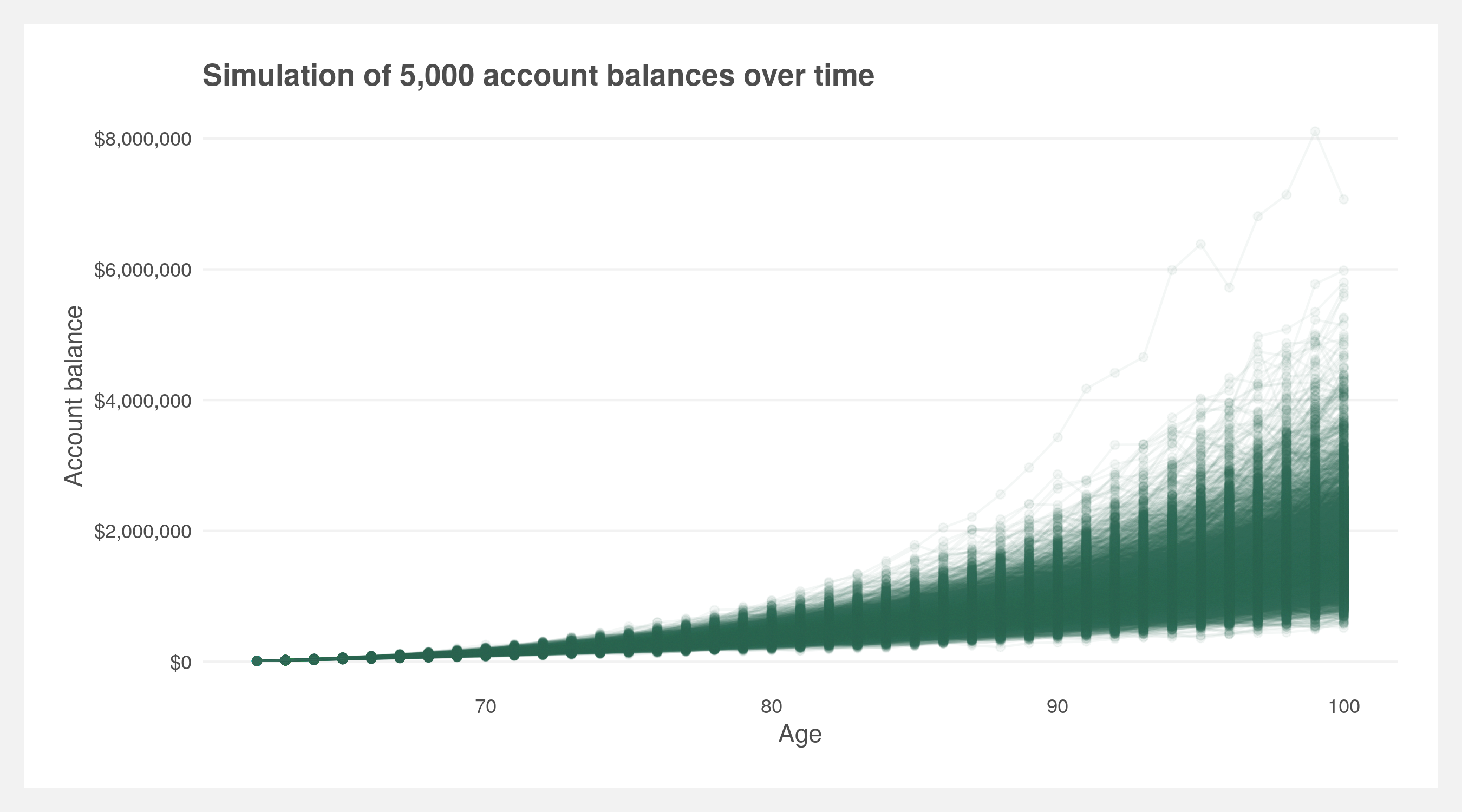
Since we are calculating the present value we only care about the final ending value. And we only need one of those 5,000 values to pick for our present value calculation. We can shoot for the middle of the road by choosing the 50th percentile or a more conservative approach would be choosing the 20th percentile — that represents the value where 80% of the other values are greater than it. Let’s do three approaches representing conservative (20th), moderate (50th), and aggressive (80th) expectations.
# set the percentile (quantile) we are interested in (lower percentile = more conservative)
percentile <- c(0.2, 0.5, 0.8)

# calculate benefits then add investment return then calculate present value
benefits$Benefits %>%
  grab_percentile_inv_return(., exp.return = exp.return, exp.vol = exp.vol,
                             n.sims = n.sims, percentile = percentile) %>%
  PV(., rate = inflation.rate, periods = 100 - 62)
[1] 486898.7 655132.3 898047.4
# calculate PV for all the combinations
sim.PV <-
  pmap(list(PV.grid$Return, PV.grid$Claim.age, PV.grid$Death.age),
       function(inv.return, age, death) {
         # calculate benefits then add investment return then calculate present value
         calculate_benefits(birth.year = 1957, claim.age = age) %>%
           filter(Age >= 62,
                  Age <= death) %>%
           pull(Benefits) %>%
           grab_percentile_inv_return(
             .,
             exp.return = inv.return,
             exp.vol = (inv.return - 1) * 2,
             n.sims = n.sims,
             percentile = percentile
           ) %>%
           PV(., rate = inflation.rate, periods = death - 62)
       })

# convert into data frame and then add columns to sim.PV
sim.PV <- data.frame(matrix(unlist(sim.PV), nrow = length(sim.PV), byrow = T))
names(sim.PV) <- paste0(percentile * 100, "th percentile of investment returns")
PV.grid <- bind_cols(PV.grid, sim.PV)
rm(sim.PV)

# plot of best claim age by investment return and death age (all claim ages)
PV.grid %>%
  select(-PV) %>%
  pivot_longer(cols = contains("percentile"), names_to = "Percentile", values_to = "PV") %>%
  group_by(Return, Death.age, Percentile) %>%
  filter(PV == max(PV)) %>%
  ggplot(aes(x = Death.age, y = Return, fill = as.factor(Claim.age))) +
  geom_tile() +
  scale_fill_brewer(name = "Claim age") +
  scale_y_continuous(breaks = seq(1, 1.1, by = 0.01),
                     labels = scales::percent(0:10/100, 1)) +
  scale_x_continuous(breaks = seq(65, 100, 5)) +
  labs(title = "Best age to claim Social Security to maximum lifetime benefits",
       subtitle = paste("Based on",
                        scales::comma(n.sims),
                        "simulations per each intersection of return, longevity, and claim age"),
       x = "Expected longevity (years)",
       y = "Expected investment return") +
  facet_wrap(~Percentile, nrow = length(percentile)) +
  light.theme +
  theme(panel.grid.major.y = element_line(color = NA),
        plot.caption = element_text(color = "gray30",
                                    face = 'italic',
                                    size = 7),
        legend.position = "bottom")
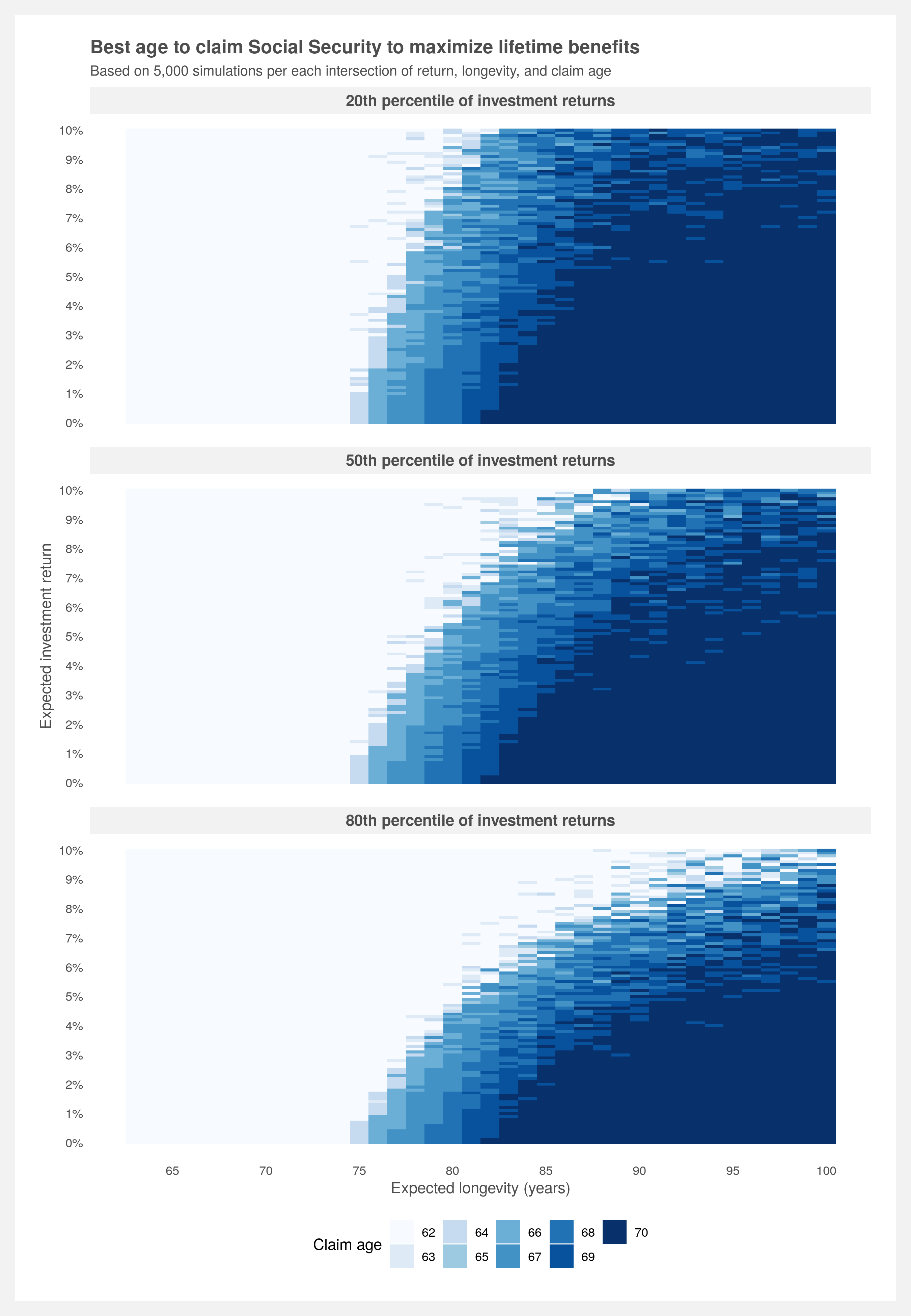
Final thoughts
I find the original deterministic plot much easier to read. The trend is clear and there’s obviously less noise. However, the takeaway from the simulated version is to lower your expectations of investment return. Therefore, if you’re going to use the deterministic version perhaps it’s best to use a lower return expectation than you would otherwise.
There are two items that could be refined for a second iteration of this project. First, the volatility assumptions for the investment simulations are simply twice the return. This is a decent estimation as volatility increases with return, however, more refined assumptions that account for specific portfolio mixtures would be best. Second, the calculator only allows claiming dates on an annual basis. The rules of Social Security allow for claiming on a monthly basis along with commensurate increases/decreases in benefits.
An addendum on vectorizing
The above investment simulation is generalizable and simple to follow but it’s resource intensive — taking up to two hours depending on your machine. As it stands, the simulation is calculating 101 x 9 x 38 x 5,000 (investment returns x claim ages x death ages x simulations) = 172,710,000 values. A faster approach would be to vectorize as much of the process as we can. Vectorizing within the simulation does not provide any speed advantages because the recursive nature of applying investment returns to incremental cashflows is difficult to simplify with vectors. However, vectorizing across simulations is possible and can provide a substantial speed increase.
The previous method repeats the following process for each of the 101 x 9 x 38 = 34,542 combinations:
- Calculate the benefits
- Simulate investing those benefits 5,000 times
- Grab the percentile ending values
- Discount the values back to today
We can cut down the calculations by >97.4% by creating a single matrix of simulated invested cashflows for each set of death ages. I.e. for each of the 101 x 9 = 909 combinations:
- Calculate the benefits to age 100
- Simulate investing those benefits 5,000 times
- Grab the percentile ending value for each age within 63:100. This represents the age of death
- Discount the resulting vector back to today
This method reduces the simulation calls from 101 x 9 x 38 = 34,542 to 101 x 8 = 909 by vectorizing across death ages. Additionally, we call the PV() function once on the whole vector of results rather than within each iteration of 101 x 9 x 39 = 34,542.
Runtime is reduced from two hours to about three minutes which is ~40x faster. Not bad for a slight tradeoff in readability.
# create all combinations of investment returns and claim age
PV.grid <- crossing(Return = seq(1, 1.1, by = 0.001),
                    Claim.age = 62:70)

# calculate quantiles for all the combinations
sim.PV <- map2_dfr(PV.grid$Return, PV.grid$Claim.age,
                   function(inv.return, age){

  # calculate the benefits
  benefits <- calculate_benefits(birth.year = 1957,
                                 claim.age = age) %>%
  filter(Age >= 62) %>%
  pull(Benefits)

  # simulate the investment returns from 62:100
  sims <- replicate(
    n.sims,
    sim_investment_return(
      cashflows = benefits,
      exp.return = inv.return,
      exp.vol = (inv.return - 1) * 2
    )
  )

  # calculate the quantiles for each death age and clean up
  quantiles <- sapply(62:100 - 61, FUN = function(death) {
    quantile(sims[death,], probs = percentile)}) %>%
    t() %>%
    as_tibble() %>%
    mutate(
      death.age = 62:100,
      claim.age = age,
      inv.return = inv.return
    )
}) %>% filter(death.age > claim.age)

# rename the percentile columns
names(sim.PV)[1:length(percentile)] <- paste0(percentile * 100, "th percentile of investment returns")

This post should not be misconstrued as financial advice. Financial planning is a highly personalized process and is best handled by a professional financial planner.
2019 December
Find the code here: github.com/joemarlo/Social-Security